Replicating the Experiments
This page provides a guide to replicate the experiments on Model Evaluation and Comparison in the OrdinoR framework paper.
Note
Before proceeding, make sure that OrdinoR has been installed. (How to install?)
Download
Download and extract the bundled zip from
this link,
navigate to folder experiment/, in which you will find the
following files and folders:
.
├── batch.py
├── configs
│   ├── bpic17.graphml
│   └── wabo.graphml
├── data.zip
├── execute.py
└── trace_clustering_reports
    ├── bpic17.bosek14.tcreport
    └── wabo.bosek5.tcreport
File data.zip contains the two event logs used in the experiments.
Folder configs/ contains the configuration files with respect to the
two logs.
Folder trace_clustering_reports/ contains the trace clustering results
generated from applying the Context Aware Trace Clustering technique
[bose2009] (“Guide Tree Miner” in ProM 6), prepared for the experiments.
Follow the steps below to conduct the experiments.
Run the Experiments
1. Prepare the experiment dataset
Extract data.zip under the current folder.
data/
├── bpic17.xes
└── wabo.xes
Note that these log files have been preprocessed accordingly, as described in the manuscript.
2. (Optional) Edit the experiment setup
Navigate to folder configs/, you will find two configuration files:
configs/
├── bpic17.graphml
└── wabo.graphml
You can choose to view and edit the configuration files with diagramming. To do so, we recommend using Gephi (other graph visualization software should suffice as long as it supports the GraphML format used for recording the configuration):
Load a configuration file with extension
.graphmlusing Gephi.(Optional) Toggle on “Show Node Labels” (by clicking on the T button on the bottom-left corner) for better visualization.
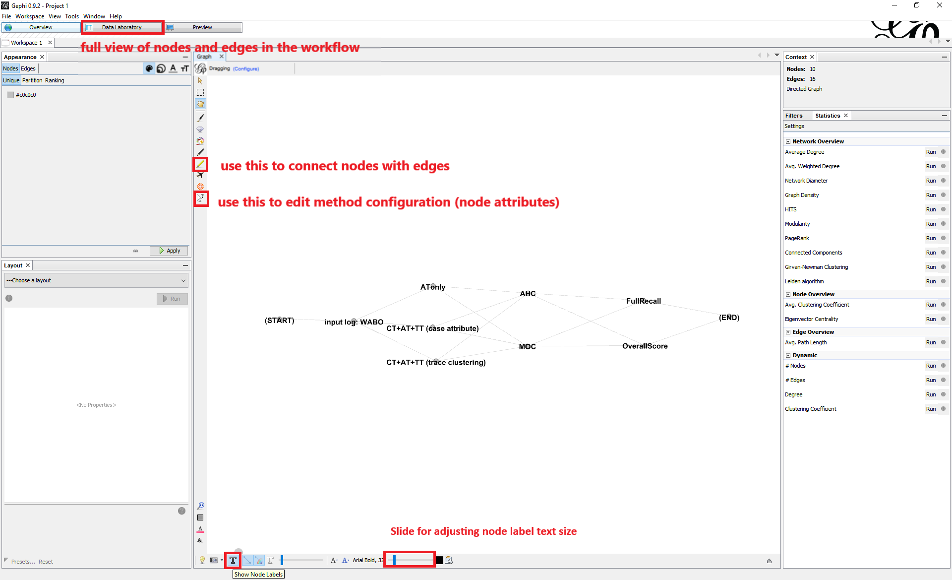
Edit the edge connections to determine which methods should be combined for model discovery.
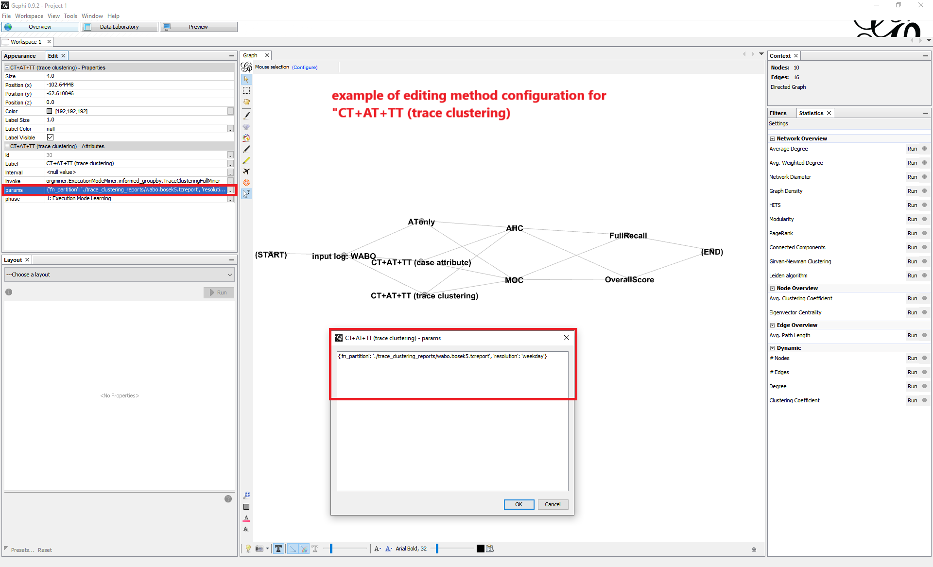
View and edit the parameter settings for each of the methods as node attributes. For a brief instruction on how to alter the parameter values, refer to Appendix: Parameter Settings.
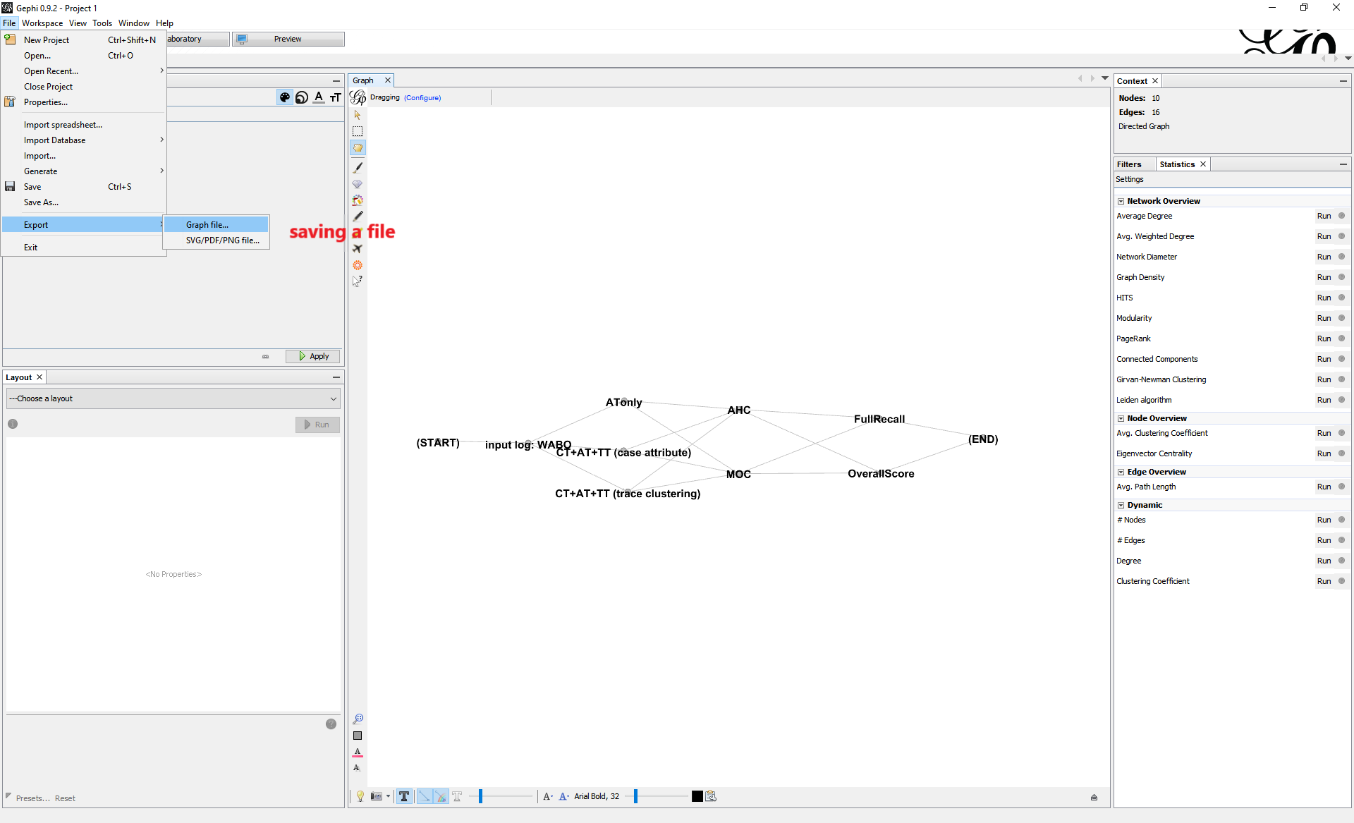
Use “File->Export->Graph file” to save the new configuration file as GraphML format.
3. Run an experiment
Note
Due to the grid search procedure and cross-validation used in the experiments, a long computation time is expected depending on the computer power. This is especially the case for log “BPIC17” in the dataset with 475,306 events.
Go to the working folder and run the program with the following command
python batch.py ./configs/wabo.graphml [<path_to_output_folder>]
with path to the output folder specified accordingly.
Change the filename to bpic17.graphml to run the experiments on
another event log.
4. Check the experiment results
The experiments will be conducted automatically according to the configuration file provided. After completion, you may find two types of files under the specified output folder:
*.om, a discovered organizational model. The filename shows the corresponding methods used for discovering this model..*_report.csv, model evaluation results of a discovered model.
Appendix: Parameter Settings
For input event log, the following parameter can be configured:
filepath: a string specifying the path to the input event log file in IEEE XES format.
For Execution Context Learning methods,
ATonly: nothing to configurable.
CT+AT+TT (case attribute):
case_attr_name, a string specifying a case-level attribute in the log used for deriving case types.resolution, a value of {'hour','day','weekday'} specifying a time unit used for deriving time types.
CT+AT+TT (trace clustering):
fn_partition, a string specifying the path to a file containing the trace clustering results on the input log.resolution, a value of {'hour','day','weekday'} specifying a time unit used for deriving time types.
For Resource Grouping discovery methods,
AHC:
n_groups: a string in the formatlist(range(x, y))specifying the range of possible number of resource groups to be searched. Substitutexandywith actual integers desired. Note that the range is defined as[x, y), i.e., non-inclusive on the right side.method, a value of {'ward','complete','average','single'} specifying the linkage criterion. See Scikit-learn AHC method for a reference.metric, a value of {'euclidean','cosine','correlation'} specifying the distance metric.
MOC:
n_groups: a string in the formatlist(range(x, y))specifying the range of possible number of resource groups to be searched. Substitutexandywith actual integers desired. Note that the range is defined as[x, y), i.e., non-inclusive on the right side.init: a value of {'random','kmeans'} specifying the strategy used for initializing the parameters of MOC. With'random', a random initialization with 100 runs is used; with'kmeans', the seed is derived from first applying the kMeans algorithm.
For Resource Group Profiling methods,
FullRecall: nothing to configure.
OverallScore:
w1: a float number in range (0, 1) specifying the weighting assigned to Group Relative Stake. When given, the weighting value assigned to Group Coverage will be determined consequently as they sum up to 1.0.p: a float number in range (0, 1) specifying the threshold value.auto_search: a Boolean value, i.e.,TrueorFalse, specifying whether or not to automatically determine the weighting values and threshold value applying grid search strategy. IfTrue, i.e., to use auto-search, then values given to'w1'and'p'will be overridden.
Report Issues
Please use the GitHub Issues page.